San Francisco Rent Analysis

Rents in San Francsisco 2000-2018
# download directly off tidytuesdaygithub repo
rent <- readr::read_csv('https://raw.githubusercontent.com/rfordatascience/tidytuesday/master/data/2022/2022-07-05/rent.csv')
What are the variable types? Do they all correspond to what they really are? Which variables have most missing values?
There are 8 character variables and 9 numeric variables. They all seem to correspond to what they really are. The variable with the most missing values is “descr”.
# YOUR CODE GOES HERE
skimr::skim(rent)| Name | rent |
| Number of rows | 200796 |
| Number of columns | 17 |
| _______________________ | |
| Column type frequency: | |
| character | 8 |
| numeric | 9 |
| ________________________ | |
| Group variables | None |
Variable type: character
| skim_variable | n_missing | complete_rate | min | max | empty | n_unique | whitespace |
|---|---|---|---|---|---|---|---|
| post_id | 0 | 1.00 | 9 | 14 | 0 | 200796 | 0 |
| nhood | 0 | 1.00 | 4 | 43 | 0 | 167 | 0 |
| city | 0 | 1.00 | 5 | 19 | 0 | 104 | 0 |
| county | 1394 | 0.99 | 4 | 13 | 0 | 10 | 0 |
| address | 196888 | 0.02 | 1 | 38 | 0 | 2869 | 0 |
| title | 2517 | 0.99 | 2 | 298 | 0 | 184961 | 0 |
| descr | 197542 | 0.02 | 13 | 16975 | 0 | 3025 | 0 |
| details | 192780 | 0.04 | 4 | 595 | 0 | 7667 | 0 |
Variable type: numeric
| skim_variable | n_missing | complete_rate | mean | sd | p0 | p25 | p50 | p75 | p100 | hist |
|---|---|---|---|---|---|---|---|---|---|---|
| date | 0 | 1.00 | 2.01e+07 | 44694.07 | 2.00e+07 | 2.01e+07 | 2.01e+07 | 2.01e+07 | 2.02e+07 | ▁▇▁▆▃ |
| year | 0 | 1.00 | 2.01e+03 | 4.48 | 2.00e+03 | 2.00e+03 | 2.01e+03 | 2.01e+03 | 2.02e+03 | ▁▇▁▆▃ |
| price | 0 | 1.00 | 2.14e+03 | 1427.75 | 2.20e+02 | 1.30e+03 | 1.80e+03 | 2.50e+03 | 4.00e+04 | ▇▁▁▁▁ |
| beds | 6608 | 0.97 | 1.89e+00 | 1.08 | 0.00e+00 | 1.00e+00 | 2.00e+00 | 3.00e+00 | 1.20e+01 | ▇▂▁▁▁ |
| baths | 158121 | 0.21 | 1.68e+00 | 0.69 | 1.00e+00 | 1.00e+00 | 2.00e+00 | 2.00e+00 | 8.00e+00 | ▇▁▁▁▁ |
| sqft | 136117 | 0.32 | 1.20e+03 | 5000.22 | 8.00e+01 | 7.50e+02 | 1.00e+03 | 1.36e+03 | 9.00e+05 | ▇▁▁▁▁ |
| room_in_apt | 0 | 1.00 | 0.00e+00 | 0.04 | 0.00e+00 | 0.00e+00 | 0.00e+00 | 0.00e+00 | 1.00e+00 | ▇▁▁▁▁ |
| lat | 193145 | 0.04 | 3.77e+01 | 0.35 | 3.36e+01 | 3.74e+01 | 3.78e+01 | 3.78e+01 | 4.04e+01 | ▁▁▅▇▁ |
| lon | 196484 | 0.02 | -1.22e+02 | 0.78 | -1.23e+02 | -1.22e+02 | -1.22e+02 | -1.22e+02 | -7.42e+01 | ▇▁▁▁▁ |
summary(rent)## post_id date year nhood
## Length:200796 Min. :20000902 Min. :2000 Length:200796
## Class :character 1st Qu.:20050227 1st Qu.:2005 Class :character
## Mode :character Median :20110924 Median :2011 Mode :character
## Mean :20095718 Mean :2010
## 3rd Qu.:20120805 3rd Qu.:2012
## Max. :20180717 Max. :2018
##
## city county price beds
## Length:200796 Length:200796 Min. : 220 Min. : 0
## Class :character Class :character 1st Qu.: 1295 1st Qu.: 1
## Mode :character Mode :character Median : 1800 Median : 2
## Mean : 2135 Mean : 2
## 3rd Qu.: 2505 3rd Qu.: 3
## Max. :40000 Max. :12
## NA's :6608
## baths sqft room_in_apt address
## Min. :1 Min. : 80 Min. :0.000 Length:200796
## 1st Qu.:1 1st Qu.: 750 1st Qu.:0.000 Class :character
## Median :2 Median : 1000 Median :0.000 Mode :character
## Mean :2 Mean : 1202 Mean :0.001
## 3rd Qu.:2 3rd Qu.: 1360 3rd Qu.:0.000
## Max. :8 Max. :900000 Max. :1.000
## NA's :158121 NA's :136117
## lat lon title descr
## Min. :34 Min. :-123 Length:200796 Length:200796
## 1st Qu.:37 1st Qu.:-122 Class :character Class :character
## Median :38 Median :-122 Mode :character Mode :character
## Mean :38 Mean :-122
## 3rd Qu.:38 3rd Qu.:-122
## Max. :40 Max. : -74
## NA's :193145 NA's :196484
## details
## Length:200796
## Class :character
## Mode :character
##
##
##
## Make a plot that shows the top 20 cities in terms of % of classifieds between 2000-2018. You need to calculate the number of listings by city, and then convert that number to a %.
# YOUR CODE GOES HERE
rent %>%
  count(city, sort=TRUE) %>%
  mutate(prop = n/sum(n)) %>%
  slice_max(order_by = prop, n=20) %>%
  mutate(city = fct_reorder(city, prop)) %>%

  ggplot(aes(x=prop, y= city)) +
  geom_col() +
  labs(title = "San Francisco accounts for more than a quarter of all rental classifieds",
       subtitle = "% of Craigslist listings, 2000-2018",
       caption = "Source: Pennington, Kate (2018). Bay Area Craigslist Rental Housing Posts, 2000-2018", y = "City", x = element_blank()) +
  scale_x_continuous(labels = scales::percent)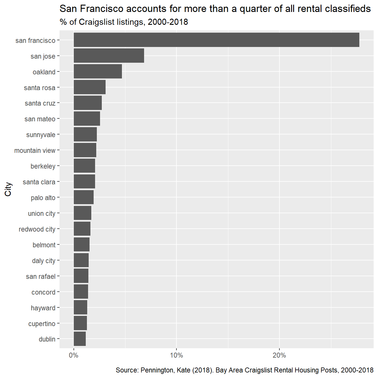
Make a plot that shows the evolution of median prices in San Francisco for 0, 1, 2, and 3 bedrooms listings.
# YOUR CODE GOES HERE
rent %>%
  filter(city == "san francisco", beds<=3) %>%
  group_by(year, beds) %>%
  summarise(median_price = median(price)) %>%

ggplot( mapping=aes(x=year, y=median_price, colour = factor(beds))) +
  geom_line() +
  facet_wrap(~beds, nrow=1)+
  theme(legend.position = "none") +
  labs(title = "San Francisco rents have been steadily increasing",
       subtitle = "0- to 3-bed listings, 2000-2018",
       caption = "Source: Pennington, Kate (2018). Bay Area Craigslist Rental Housing Posts, 2000-2018", y = element_blank(), x = element_blank())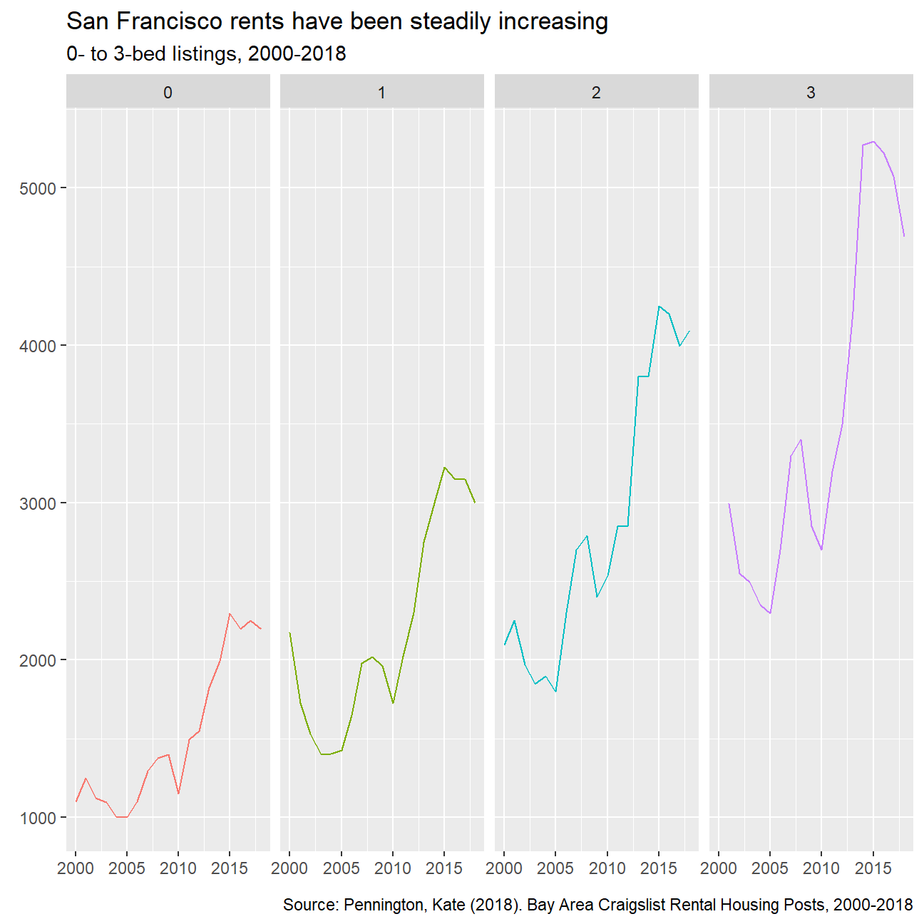
Finally, make a plot that shows median rental prices for the top 12 cities in the Bay area.
# YOUR CODE GOES HERE
rent %>%
  filter(city %in% c("san francisco", "san jose", "oakland", "santa rosa", "santa cruz", "san mateo", "sunnyvale", "mountain view", "berkeley", "santa clara", "palo alto", "union city"), beds == 1)%>%
  group_by(city,year) %>%
  summarise(median_price = median(price), city)%>%

  ggplot(aes(x=year, y=median_price, color=city)) +
  geom_line() +
  facet_wrap(~city, nrow=3)+
  theme(legend.position = "none") +
  labs(title = "Median rental prices for 1 bedroom flats in top 12 cities from Bay Area", x = "Year", y = "Median rental price", caption = "Source: Pennington, Kate (2018). Bay Area Craigslist Rental Housing Posts, 2000-2018")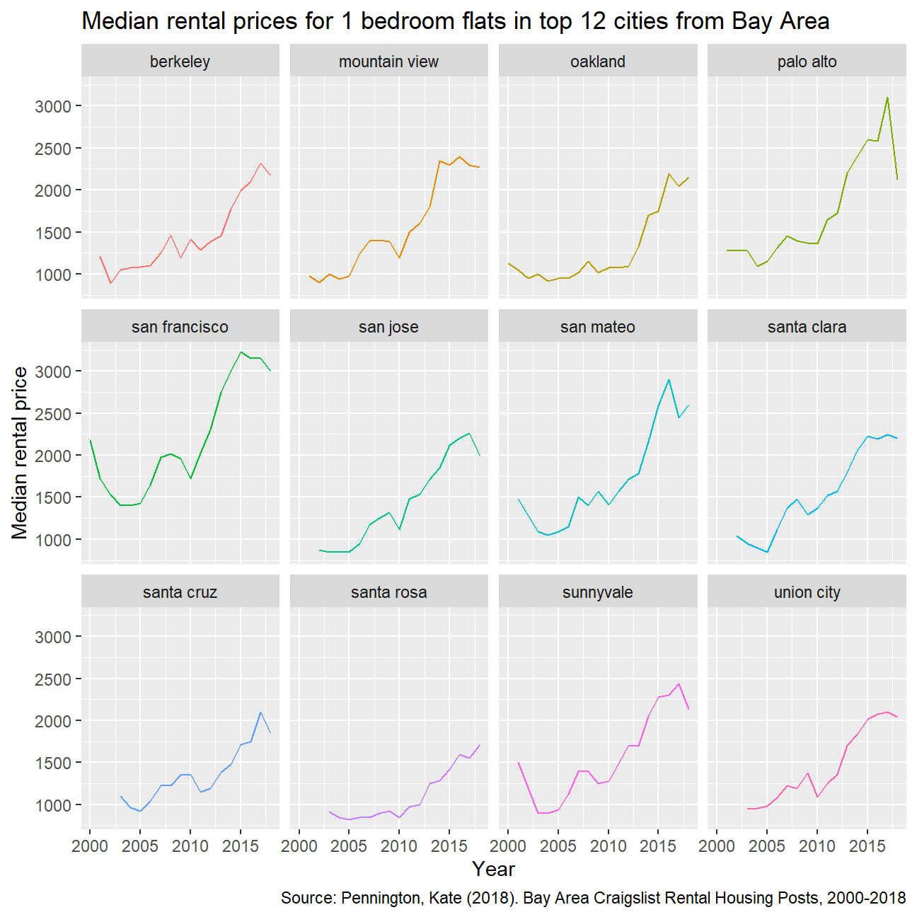
What can you infer from these plots? Don’t just explain what’s in the graph, but speculate or tell a short story (1-2 paragraphs max).
The general trend that can be seen across the cities in the Bay area is that the rent has decreased in the years following the dot.com bubble (2001-2004), after which it increased rapidly prior to the housing market crash and global financial crisis that started in 2007-2008. After 2010 rents started increasing rapidly again until the economic slowdown that commenced at the end of the decade.